Air-Standard Brayton Cycle Example

Imports

from thermostate import State, Q_, units
from thermostate.plotting import IdealGas
import numpy as np

%matplotlib inline
import matplotlib.pyplot as plt

---

Definitions

substance = "air"
p_1 = Q_(1.0, "bar")
T_1 = Q_(300.0, "K")
T_3 = Q_(1700.0, "K")
p2_p1 = Q_(8.0, "dimensionless")
p_low = Q_(2.0, "dimensionless")
p_high = Q_(50.0, "dimensionless")

---

Problem Statement

An ideal air-standard Brayton cycle operates at steady state with compressor inlet conditions of 300.0 K and 1.0 bar and a fixed turbine inlet temperature of 1700.0 K and a compressor pressure ratio of 8.0. For the cycle,

1. determine the net work developed per unit mass flowing, in kJ/kg

2. determine the thermal efficiency

3. plot the net work developed per unit mass flowing, in kJ/kg, as a function of the compressor pressure ratio from 2.0 to 50.0

4. plot the thermal efficiency as a function of the compressor pressure ratio from 2.0 to 50.0

5. Discuss any trends you find in parts 3 and 4

---

Solution

1. the net work developed per unit mass flowing

The ideal Brayton cycle is made of 4 processes:

1. Isentropic compression
2. Isobaric heat input
3. Isentropic expansion
4. Isobaric heat rejection

The following properties are used to fix the four states:

State	Property 1	Property 2
1	\[T_1\]	\[p_1\]
2	\[p_2\]	\[s_2=s_1\]
3	\[p_3=p_2\]	\[T_3\]
4	\[s_4=s_3\]	\[p_4=p_1\]

In the ideal Brayton cycle, work occurs in the isentropic compression and expansion. Therefore, the works are

\[\begin{aligned} \frac{\dot{W}_c}{\dot{m}} &= h_1 - h_2 & \frac{\dot{W}_t}{\dot{m}} &= h_3 - h_4 \end{aligned}\]

First, fixing the four states

st_1 = State(substance, T=T_1, p=p_1)
h_1 = st_1.h.to("kJ/kg")
s_1 = st_1.s.to("kJ/(kg*K)")

s_2 = s_1
p_2 = p_1 * p2_p1
st_2 = State(substance, p=p_2, s=s_2)
h_2 = st_2.h.to("kJ/kg")
T_2 = st_2.T

p_3 = p_2
st_3 = State(substance, p=p_3, T=T_3)
h_3 = st_3.h.to("kJ/kg")
s_3 = st_3.s.to("kJ/(kg*K)")

s_4 = s_3
p_4 = p_1
st_4 = State(substance, p=p_4, s=s_4)
h_4 = st_4.h.to("kJ/kg")
T_4 = st_4.T

Summarizing the states,

State	T	p	h	s
1	300.00 K	1.00 bar	426.30 kJ/kg	3.89 kJ/(K kg)
2	540.13 K	8.00 bar	670.65 kJ/kg	3.89 kJ/(K kg)
3	1700.00 K	8.00 bar	2007.09 kJ/kg	5.19 kJ/(K kg)
4	1029.42 K	1.00 bar	1206.17 kJ/kg	5.19 kJ/(K kg)

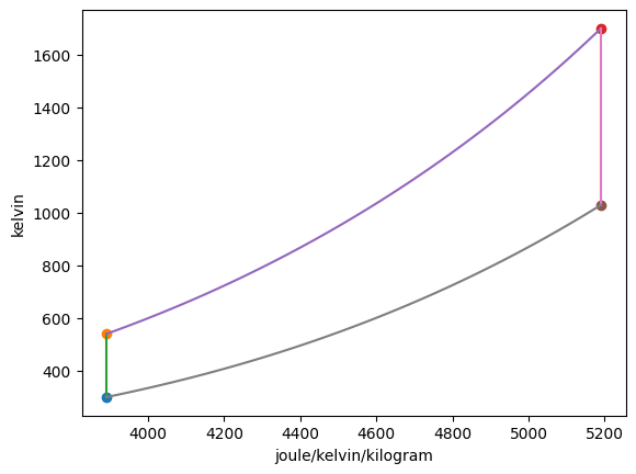
Plotting the p-v and T-s diagrams of the cycle,

Brayton = IdealGas(substance, ("s", "T"), ("v", "p"))

Brayton.add_process(st_1, st_2, "isentropic")
Brayton.add_process(st_2, st_3, "isobaric")
Brayton.add_process(st_3, st_4, "isentropic")
Brayton.add_process(st_4, st_1, "isobaric")

Then, the net work is calculated by

W_c = h_1 - h_2
W_t = h_3 - h_4
W_net = W_c + W_t

Answer: The works are \(\dot{W}_c/\dot{m} =\) -244.35 kJ/kg, \(\dot{W}_t/\dot{m} =\) 800.92 kJ/kg, and \(\dot{W}_{net}/\dot{m} =\) 556.57 kJ/kg

2. the thermal efficiency

Q_23 = h_3 - h_2
eta = W_net / Q_23

Answer: The thermal efficiency is \(\eta =\) 0.42 = 41.65%

3. and 4. plot the net work per unit mass flowing and thermal efficiency

p_range = np.linspace(p_low, p_high, 50)
eta_l = np.zeros(shape=p_range.shape) * units.dimensionless
W_net_l = np.zeros(shape=p_range.shape) * units.kJ / units.kg
for i, p_ratio in enumerate(p_range):
    s_2 = s_1
    p_2 = p_1 * p_ratio
    st_2 = State(substance, p=p_2, s=s_2)
    h_2 = st_2.h.to("kJ/kg")
    T_2 = st_2.T

    p_3 = p_2
    st_3 = State(substance, p=p_3, T=T_3)
    h_3 = st_3.h.to("kJ/kg")
    s_3 = st_3.s.to("kJ/(kg*K)")

    s_4 = s_3
    p_4 = p_1
    st_4 = State(substance, p=p_4, s=s_4)
    h_4 = st_4.h.to("kJ/kg")
    T_4 = st_4.T

    W_c = h_1 - h_2
    W_t = h_3 - h_4
    W_net = W_c + W_t
    W_net_l[i] = W_net

    Q_23 = h_3 - h_2
    eta = W_net / Q_23
    eta_l[i] = eta

fig, work_ax = plt.subplots()
work_ax.plot(p_range, W_net_l, label="Net work per unit mass flowing", color="C0")
eta_ax = work_ax.twinx()
eta_ax.plot(p_range, eta_l, label="Thermal efficiency", color="C1")
work_ax.set_xlabel("Pressure ratio $p_2/p_1$")
work_ax.set_ylabel("Net work per unit mass flowing (kJ/kg)")
eta_ax.set_ylabel("Thermal efficiency")
lines, labels = work_ax.get_legend_handles_labels()
lines2, labels2 = eta_ax.get_legend_handles_labels()
work_ax.legend(lines + lines2, labels + labels2, loc="best");

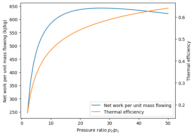
We note from this graph that the thermal efficiency of the cycle increases continuously as the pressure ratio increases. However, because there is a fixed turbine inlet temperature, the work per unit mass flowing has a maximum around \(p_2/p_1\) = 20.