Cold-Air Standard Brayton Cycle Example

Imports

from thermostate import State, Q_, units
import numpy as np

%matplotlib inline
import matplotlib.pyplot as plt

---

Definitions

substance = "air"
p_1 = Q_(1.0, "bar")
T_1 = Q_(300.0, "K")
mdot = Q_(6.0, "kg/s")
T_3 = Q_(1400.0, "K")
p2_p1 = Q_(10.0, "dimensionless")
T_3_low = Q_(1000.0, "K")
T_3_high = Q_(1800.0, "K")

---

Problem Statement

An ideal cold air-standard Brayton cycle operates at steady state with compressor inlet conditions of 300.0 kelvin and 1.0 bar and a fixed turbine inlet temperature of 1400.0 kelvin and a compressor pressure ratio of 10.0 dimensionless. The mass flow rate of the air is 6.0 kilogram / second. For the cycle,

1. determine the back work ratio

2. determine the net power output, in kW

3. determine the thermal efficiency

4. plot the net power output, in kW, and the thermal efficiency, as a function of the turbine inlet temperature from 1000.0 kelvin to 1800.0 kelvin. Discuss any trends you find.

---

Solution

1. the back work ratio

In the ideal Brayton cycle, work occurs in the isentropic compression and expansion. Therefore, the works are

\[\begin{aligned} \frac{\dot{W}_c}{\dot{m}} &= h_1 - h_2 = c_p(T_1 - T_2) & \frac{\dot{W}_t}{\dot{m}} &= h_3 - h_4 = c_p(T_3 - T_4) \end{aligned}\]

First, fixing the four states using a cold air-standard analysis

st_amb = State(substance, T=T_1, p=p_1)
c_v = st_amb.cv
c_p = st_amb.cp
k = c_p / c_v

T_2 = T_1 * p2_p1 ** ((k - 1) / k)
p_2 = p2_p1 * p_1

p_3 = p_2

p_4 = p_1
T_4 = T_3 * (p_4 / p_3) ** ((k - 1) / k)

Summarizing the states,

State	T	p
1	300.00 K	1.00 bar
2	580.34 K	10.00 bar
3	1400.00 K	10.00 bar
4	723.71 K	1.00 bar

Then, the back work ratio can be found by

Wdot_c = (mdot * c_p * (T_1 - T_2)).to("kW")
Wdot_t = (mdot * c_p * (T_3 - T_4)).to("kW")
bwr = abs(Wdot_c) / Wdot_t

Answer: The power outputs are \(\dot{W}_c =\) -1692.75 kW, \(\dot{W}_t =\) 4083.53 kW, and the back work ratio is \(\mathrm{bwr} =\) 0.41 = 41.45%

2. the net power output

Wdot_net = Wdot_c + Wdot_t

Answer: The net power output is \(\dot{W}_{net} =\) 2390.78 kW

3. the thermal efficiency

Qdot_23 = (mdot * c_p * (T_3 - T_2)).to("kW")
eta = Wdot_net / Qdot_23

Answer: The thermal efficiency is \(\eta =\) 0.48 = 48.31%

4. plot the net power output and thermal efficiency

T_range = np.linspace(T_3_low, T_3_high, 200)
Wdot_net_l = np.zeros(T_range.shape) * units.kW
eta_l = np.zeros(T_range.shape) * units.dimensionless
for i, T_3 in enumerate(T_range):
    T_4 = T_3 * (p_4 / p_3) ** ((k - 1) / k)
    Wdot_t = (mdot * c_p * (T_3 - T_4)).to("kW")
    Wdot_net = Wdot_c + Wdot_t
    Wdot_net_l[i] = Wdot_net

    Qdot_23 = (mdot * c_p * (T_3 - T_2)).to("kW")
    eta = Wdot_net / Qdot_23
    eta_l[i] = eta

fig, power_ax = plt.subplots()
power_ax.plot(T_range, Wdot_net_l, label="Net power output", color="C0")
eta_ax = power_ax.twinx()
eta_ax.plot(T_range, eta_l, label="Thermal efficiency", color="C1")
power_ax.set_xlabel("Turbine Inlet Temperature (K)")
power_ax.set_ylabel("Net power output (kW)")
eta_ax.set_ylabel("Thermal efficiency")
lines, labels = power_ax.get_legend_handles_labels()
lines2, labels2 = eta_ax.get_legend_handles_labels()
power_ax.legend(lines + lines2, labels + labels2, loc="best");

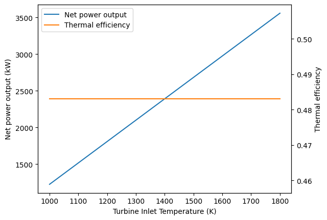
From this graph, we note that for a fixed compressor pressure ratio, the thermal efficiency is constant, while the net power output increases with increasing turbine temperature.