Cascade Refrigeration Cycle Example

Imports

from thermostate import State, Q_, units, EnglishEngineering as EE
from thermostate.plotting import IdealGas, VaporDome

---

Definitions

sub_hiT = "R22"
sub_loT = "R134A"

T_1 = Q_(-30.0, "degF")
x_1 = Q_(1.0, "dimensionless")

p_2 = Q_(50.0, "psi")

p_3 = p_2
x_3 = Q_(0.0, "dimensionless")

delta_T_5 = Q_(-5.0, "delta_degF")
x_5 = Q_(1.0, "dimensionless")

p_6 = Q_(250.0, "psi")

p_7 = p_6
x_7 = Q_(0.0, "dimensionless")

Qdot_in = Q_(20.0, "refrigeration_tons")

---

Problem Statement

A two-stage cascade vapor-compression refrigeration system operates with R22 as the working fluid in the high-temperature cycle and R134A in the low-temperature cycle. For the R134A cycle, the working fluid enters the compressor as a saturated vapor at -30.0 fahrenheit and is compressed isentropically to 50 lbf/in.2 Saturated liquid leaves the intermediate heat exchanger at 50 lbf/in.2 and enters the expansion valve. For the R22 cycle, the working fluid enters the compressor as saturated vapor at a temperature 5 fahrenheit below that of the condensing temperature of the R134A in the intermediate heat exchanger. The R22 is compressed isentropically to 250 lbf/in.2 Saturated liquid then enters the expansion valve at 250 lbf/in.2. The refrigerating capacity of the cascade system is 20 ton_of_refrigeration. Determine

1. the power input to each compressor, in BTU/min

2. the overall coefficient of performance of the cascade cycle

---

Solution

1. the power input to each compressor

The power input to each compressor can be found by

\[\dot{W}_{cv} = \dot{m}(h_i - h_e)\]

To find the enthalpies, we need to fix all of the states.

The cascade refrigeration cycle is consistes of two smaller cycles both with 4 processes:

R22 cycle:
1. Isentropic compression
2. Isobaric heat exchange
3. Isoenthalpic expansion
4. Isobaric heat exchange

R134A cycle:
1. Isentropic compression
2. Isobaric heat exchange
3. Isoenthalpic expansion
4. Isobaric heat exchange

The following properties are used to fix the four states:

State	Property 1	Property 2
1	\[x_1\]	\[T_1\]
2	\[p_2\]	\[s_2=s_1\]
3	\[p_3=p_2\]	\[x_3\]
4	\[p_4=p_1\]	\[h_4=h_3\]
5	\[T_5=T_3 + \Delta T_5\]	\[x_5\]
6	\[p_6\]	\[s_6=s_5\]
7	\[p_7=p_6\]	\[x_7\]
8	\[p_8=p_5\]	\[h_8=h_7\]

st_1 = State(sub_loT, x=x_1, T=T_1)
h_1 = st_1.h.to(EE.h)
s_1 = st_1.s.to(EE.s)
p_1 = st_1.p.to(EE.p)

s_2 = s_1
st_2 = State(sub_loT, p=p_2, s=s_1)
h_2 = st_2.h.to(EE.h)
T_2 = st_2.T.to(EE.T)

st_3 = State(sub_loT, p=p_3, x=x_3)
T_3 = st_3.T.to(EE.T)
h_3 = st_3.h.to(EE.h)
s_3 = st_3.s.to(EE.s)

h_4 = h_3
p_4 = p_1
st_4 = State(sub_loT, p=p_4, h=h_4)
T_4 = st_4.T.to(EE.T)
s_4 = st_4.s.to(EE.s)
x_4 = st_4.x

T_5 = T_3 + delta_T_5
st_5 = State(sub_hiT, T=T_5, x=x_5)
h_5 = st_5.h.to(EE.h)
p_5 = st_5.p.to(EE.p)
s_5 = st_5.s.to(EE.s)

s_6 = s_5
st_6 = State(sub_hiT, s=s_6, p=p_6)
h_6 = st_6.h.to(EE.h)
T_6 = st_6.T.to(EE.T)

st_7 = State(sub_hiT, p=p_7, x=x_7)
T_7 = st_7.T.to(EE.T)
h_7 = st_7.h.to(EE.h)
s_7 = st_7.s.to(EE.s)

h_8 = h_7
p_8 = p_5
st_8 = State(sub_hiT, p=p_8, h=h_8)
T_8 = st_8.T.to(EE.T)
s_8 = st_8.s.to(EE.s)
x_8 = st_8.x

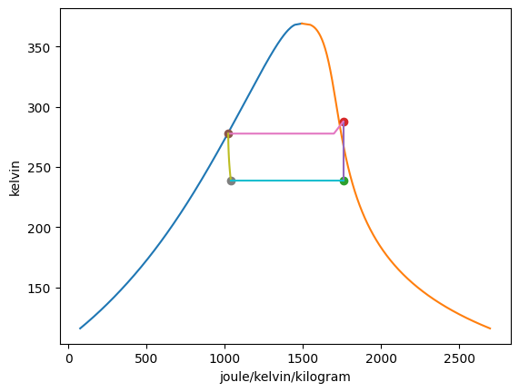
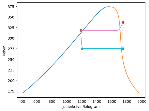
Plotting the T-s diagrams of both cycles,

R22_vapordome = VaporDome(sub_hiT, ("s", "T"))
R134A_vapordome = VaporDome(sub_loT, ("s", "T"))

R22_vapordome.add_process(st_1, st_2, "isentropic")
R22_vapordome.add_process(st_2, st_3, "isobaric")
R22_vapordome.add_process(st_3, st_4, "isoenthalpic")
R22_vapordome.add_process(st_4, st_1, "isobaric")

R134A_vapordome.add_process(st_5, st_6, "isentropic")
R134A_vapordome.add_process(st_6, st_7, "isobaric")
R134A_vapordome.add_process(st_7, st_8, "isoenthalpic")
R134A_vapordome.add_process(st_8, st_5, "isobaric")

Summarizing the states:

State	T	p	h	s	x	phase
1	-30.00 degF	9.86 pound_force_per_square_inch	162.30 btu / pound	0.4196 btu / degR / pound	100.00%	twophase
2	58.23 degF	50.00 pound_force_per_square_inch	176.42 btu / pound	0.4196 btu / degR / pound	—	gas
3	40.27 degF	50.00 pound_force_per_square_inch	88.65 btu / pound	0.2442 btu / degR / pound	0.00%	twophase
4	-30.00 degF	9.86 pound_force_per_square_inch	88.65 btu / pound	0.2482 btu / degR / pound	22.96%	twophase
5	35.27 degF	76.59 pound_force_per_square_inch	174.42 btu / pound	0.4175 btu / degR / pound	100.00%	twophase
6	146.75 degF	250.00 pound_force_per_square_inch	187.12 btu / pound	0.4175 btu / degR / pound	—	gas
7	112.76 degF	250.00 pound_force_per_square_inch	110.14 btu / pound	0.2834 btu / degR / pound	0.00%	twophase
8	35.27 degF	76.59 pound_force_per_square_inch	110.14 btu / pound	0.2876 btu / degR / pound	26.55%	twophase

The mass flow rate of the R134a is found from the refrigeration capacity

\[\dot{m}_{\text{R134A}} = \frac{\dot{Q}_{in}}{h_1 - h_4}\]

while the mass flow rate of the R22 is found from the intermediate heat exchanger

\[\dot{m}_{\text{R22}} = \frac{\dot{m}_{\text{R134A}}\left(h_2 - h_3\right)}{h_5 - h_8}\]

mdot_r134a = (Qdot_in / (h_1 - h_4)).to("lb/min")
Wdot_loT = (mdot_r134a * (h_1 - h_2)).to("BTU/min")

mdot_r22 = mdot_r134a * (h_2 - h_3) / (h_5 - h_8)
Wdot_hiT = (mdot_r22 * (h_5 - h_6)).to("BTU/min")

Answer: The compressor work for the low-temperature cycle is \(\dot{W}_{\text{R134A}} =\) -766.52 btu / minute and the work for the high temperature cycle is \(\dot{W}_{\text{R22}} =\) -941.38 btu / minute

2. The coefficient of performance

The coefficient of performance of this refrigeration cycle is defined as

\[\beta = \frac{\dot{Q}_{in}}{\lvert\dot{W}_{\text{R134A}} + \dot{W}_{\text{R22}}\rvert}\]

beta = (Qdot_in / abs(Wdot_loT + Wdot_hiT)).to("dimensionless")
beta_max = (T_4 / (T_7 - T_4)).to("dimensionless")

Answer: The coefficient of performance is \(\beta =\) 2.34, while the maximum coefficient of performance for a refrigeration cycle operating between \(T_C =\) -30.00 degF and \(T_H =\) 112.76 degF is \(\beta_{\text{max}} =\) 3.01 dimensionless. The actual cycle has a lower COP, so it is possible.